A/B testing With Alteryx (Part 2)
Data and Cloud Person
The Business Problem
Round Roasters is an upscale coffee chain with locations in the western United States of America. The past few years have resulted in stagnant growth at the coffee chain, and a new management team was put in place to reignite growth at their stores. The first major growth initiative is to introduce gourmet sandwiches to the menu, along with limited wine offerings. The new management team believes that a television advertising campaign is crucial to driving people into the stores with these new offerings. However, the television campaign will require a significant boost in the company’s marketing budget, with an unknown return on investment (ROI).
Additionally, there is concern that current customers will not buy into the new menu offerings. To minimise risk, the management team decides to test the changes in two cities with new television advertising. Denver and Chicago cities were chosen to participate in this test because the stores in these two cities (or markets) perform similarly to all stores across the entire chain of stores; performance in these two markets would be a good proxy to predict how well the updated menu performs. The test ran for 12 weeks (2016-April-29 to 2016-July-21) where five stores in each of the test markets offered the updated menu along with television advertising. To carry out our analysis we have three datasets:
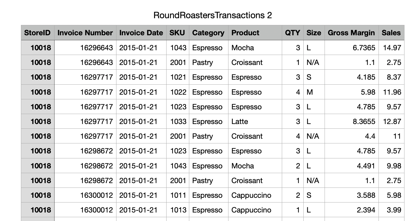
Transaction data for all stores from 2015-January-21 to 2016-August-18
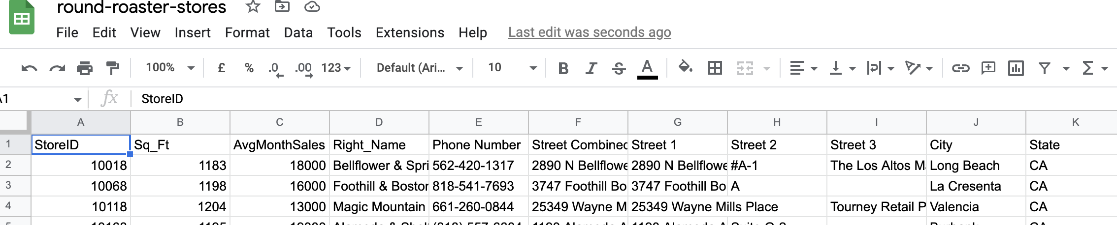
A listing of all Round Roasters stores
A listing of the 10 stores (5 in each market) that were used as test markets. I wrote a detailed introduction to A/b testing and Alteryx here.
Understanding the Experiment
First of all, this is going to be a matched pair experiment, i.e the test stores have to be matched to control stores on a unit-by-unit basis using control variables. This is because the numbers of stores are not too large and the tendency for bias is large, we want to ensure that stores with similar characteristics are matched to one another so that we can increase confidence in our results as much as possible. Matched pairing sets up treatment and control groups for experiments by matching them on a unit-by-unit basis using Control variables.
Planning the Analysis
To perform correct analysis, we need to prepare the data, but before we prepare the data, by answering some questions.
- First, what is the performance metric to evaluate the result of the test?: This is important because the performance metric is the yardstick with which we will evaluate the results of the test. In this case, the performance metric is the gross margin, the difference or the lift in the gross margin. We need to achieve at least an 18% increase in the gross margin in the control stores to justify the addition of the new additions to the Menu.
What is the test period?: The test period is 12 weeks, from the 29th of April 2016 to the 21st of July 2016
At what level should the data be aggregated?: The data should be aggregated at the weekly level.
Cleaning the data: Now that we have answered some key questions about our data, we need to format our data. First, we filter the date to only the date within the range of the test period, then we create a week column and aggregate the sum of gross margin weekly per store. Also because the transaction data contains the data for both the Control and treatment stores, we filter out the transactions for the treatment stores separately.
Matching the Stores: Now we match the Control Stores with the treatment stores, there are 10 treatment stores and 20 control stores. We will match the stores based on seasonality and treatment and some variables in our dataset; In our dataset, we have the following features: StoreID, Sq_Ft, AvgMonthSales, Right_Name, Phone Number, Street Combined, Street 1, Street 2, Street 3, City, State, Postal Code, Region, Country, Coordinates, Latitude, Longitude, Timezone, Current Timezone Offset, Olson Timezone.
Looking at these features, we can use eliminate those that will not be a suitable to match the stores. The suitable ones are on are Sq_Ft(size) and AvgMonthSales(average monthly Sales), I will check the correlation of both features with the gross margin to confirm if they are suitable.
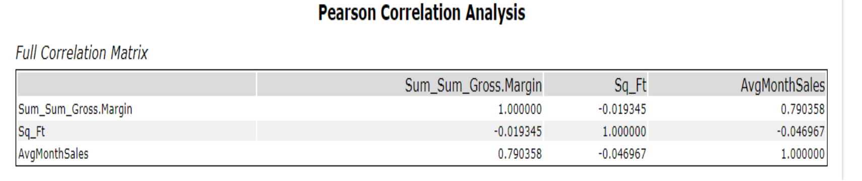
Only the average monthly Sales is correlated with the gross margin so I will be using it to match the stores. We will use the A/B trends tool in Alteryx to calculate seasonality and trend and then the A/B test tool to carry out the A/B testing as shown below:
Analyzing the results
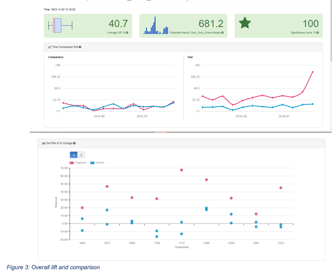
Let us break down the results into parts to understand what each part means.
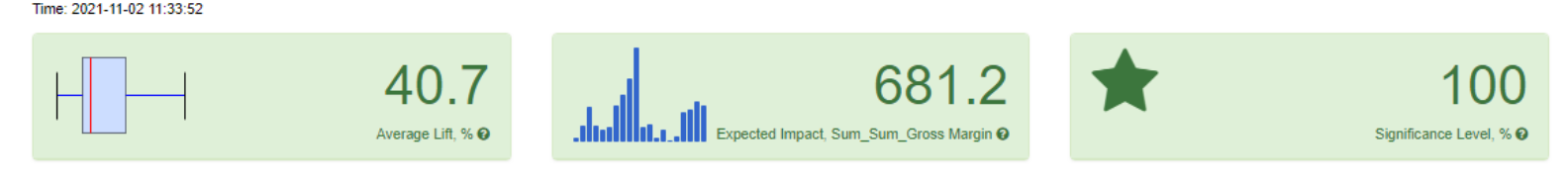
The figure at the left shows the lift in gross sum margin, the lift tells us by how much the treatment group has changed to the control group, Lift can be positive or negative, the lift is at 40.7%, which means that on average stores in the treatment group recorded a gross margin of more than 40% over the control group i.e an increase in gross margin. The middle figure tells us by how much the gross margin in the treatment store increased per week at the treatment stores. The figure at the right is the Statistical Significance. Statistical significance is used to estimate the probability of our results being due to chance. In analytical situations like this, there is an ever-present probability that the change we have seen in our test is due to chance, a statistical significance value helps to determine how confident we should be in the results of our test, a score of 100% tells us that the changes we have gotten from our test is very significant and not due to chance or random.
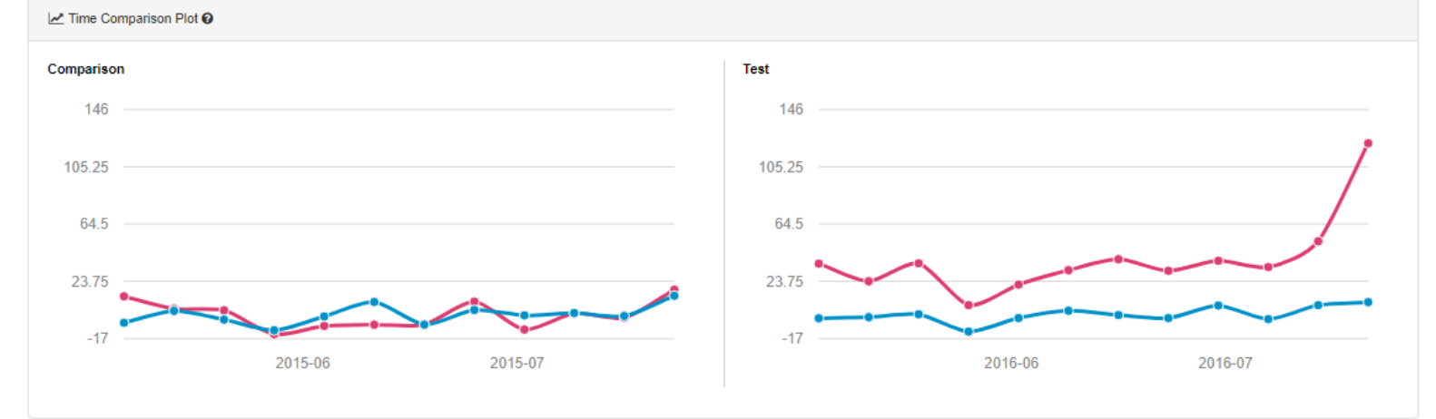
The second part of the chart compares the sales at the stores for both the treatment stores and the control stores before the test period and after the test period.
As we can see, before the test period on the left, both sets of stores were performing almost similarly, but during the test period, all treatment stores recorded higher sales numbers than the control stores.
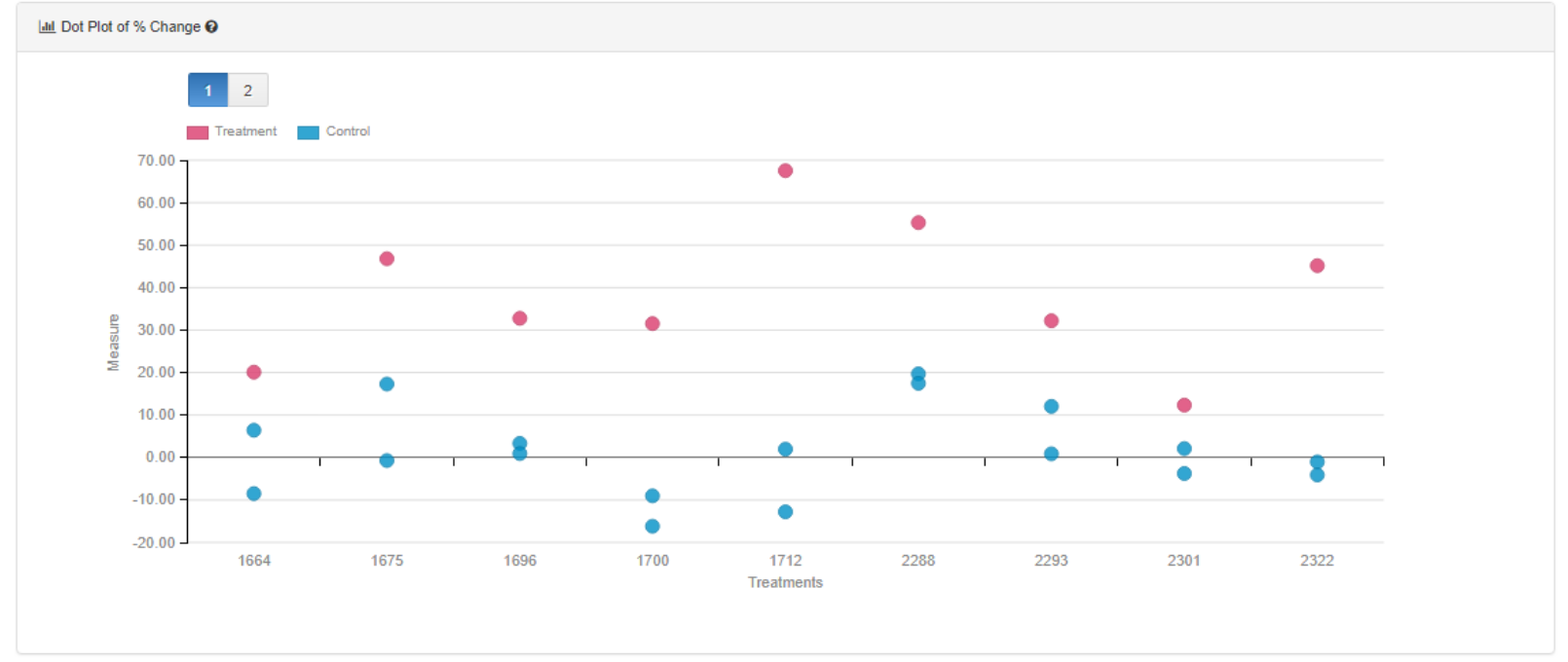
The last chart also reinforced what we have been observing so far, all the treatment stores outperformed their assigned control stores during the test period.
Conclusion and Recommendation
From the above analysis, we can recommend that the company roll out its new Menu across all its stores. The decision will not only revitalize the Menu at the stores but will also be profitable for the company.